Live Displays
The LiveDisplays plug-in allows real-time visualisation
histograms, based on pointers to TH1D and TH2D objects (see the ROOT web pages for documentation on these).
The live displays are created and initialised at run-time, can be updated
in real time as the run progresses, and can be saved to a
variety of graphics and data formats both during and after the run.
Auxiliary methods allow to include comparisons to reference
data from experimental measurements and/or saved runs, using file
read-in methods which are adaptible to almost any
conceivable (simple) column-based data format, in particular those
used by the HepDATA repository.
If the binning of the reference data differs
from that of the base TH1D object, a flag can be set to show a
rebinned version of the latter instead, recasting it into the binning
of the reference measurement.
It is also
possible to include and display a variety of additional content
including uncertainty variations, basic chi-squared
calculations, ratios, and to re-initialise/recover from previous runs.
Note: for help on ROOT, please consult the ROOT documentation and forums,
not the PYTHIA authors. Few of us are ROOT users and none of us are
ROOT developers, therefore this plug-in is provided "as is" and
any non-PYTHIA-specific questions or problems you may
encounter when using or linking this plug-in to ROOT should be addressed
to the ROOT development team.
Reference
If you use plots created by the LiveDisplays plugin
in a publication, we ask that you include a reference to [GKS11]
in which the functionality underlying the this plug-in
was first developed. It would also be appropriate to include a
reference to the ROOT software package, which the plug-in is based
on.
Disclaimer
The PYTHIA collaboration is providing this plug-in as a simple
utility for real-time histogram monitoring, which can also be used as
a convenient way to produce near-publication-quality plots. Developing
this facility is, however, not the core focus of our
collaboration, and is provided "as is". Please do
not send us any unsolicited "feature requests".
For extensions or bug fixes that are of general interest, feel free to
develop further capabilities and send us (documented and complete)
examples of working and validated code, following the CODINGSTYLE
guidelines that are distributed with PYTHIA 8, with the proviso that
we still reserve the right to make the final judgement whether
contributed code is of a sufficient quality and generality to be
included in the distributed version of the plug-in.
Finally, we emphasize that the PYTHIA collaboration is providing this plug-in
without any guarantees, explicit or implied. It is up to the user to
cross check that the graphics produced by this plug-in accurately
reflect the underlying histogram contents.
Configuration, Compilation, and Linking
To use the LiveDisplays functionality, linking
to ROOT must be enabled, using the --with-root=...
configuration option. Note also that the LiveDisplays plug-in requires
that the linked version of ROOT must be at least v.6+ (e.g., our use
of transparency is not backwards compatible with ROOT v.5.)
Once you have configured and compiled PYTHIA 8 with these options
successfully, you can check whether the plug-in works by seeing if you
can compile and execute the mainXX.cc example program in PYTHIA's
examples/ subdirectory.
We note that it is important that your ROOT libraries were compiled
with the same C++ compiler version (or at least a compatible one)
as the PYTHIA 8 (and LiveDisplays) libraries were.
Otherwise you may get errors related to inconsistent
architectures. We kindly ask you not to use us as a helpdesk
for troubleshooting problems of this kind.
The LiveDisplayApp object
In each main program that uses the LiveDisplays plugin,
a single LiveDisplaysApp
instance must be created. This takes care of defining the ROOT
TApplication instance that handles communication with the computer's
graphics display(s), and basic initialisation.
Note: only a single LiveDisplaysApp instance should be created per
main program.
Creating LiveDisplay objects
We assume that the user has already defined a TH1D (or TH2D) object,
which they intend to fill during the run. For example:
- TH1D myH1D("myHist","My Title",100,0.,1.0);
- // Optionally also set histogram axis labels and plot range
- myH1D.GetXaxis()->SetTitle("x");
- myH1D.GetYaxis()->SetTitle("f(x)");
- myH1D.SetMinimum(0.0005);
- myH1D.SetMaximum(90.);
A run-time display can be created from a TH1D (or TH2D) object,
using one of the following
three constructors (assuming that one instance of a
LiveDisplaysApp has already been created, see above):
- // 1) Construct a run-time display from a TH1D pointer:
- LiveDisplay(TH1D* th1dPtr, Pythia8::Settings* settingsPtr)
- // 2) Construct a run-time display from a TH2D pointer:
- LiveDisplay(TH2D* th2dPtr, Pythia8::Settings* settingsPtr)
- // 3) Construct a run-time display from a vector of TH1D pointers:
- LiveDisplay(vector th1dPtrList, Pythia8::Settings*
settingsPtr)
The 3rd type of constructor allows to show a band defined by the
envelope of several TH1D histograms, for instance as obtained by
filling separate TH1D histograms with different uncertainty
variations, or with different
PDF weights, etc. It is then also possible to include an additional
pane in the display, underneath the main plot pane,
showing the breakdown of relative deviations member by member in the
vector although this functionality is currently limited to up to 8
members. This pane can be enabled/disabled by the following flag:
flag LiveDisplays:showRelUnc
(default = on)
of histograms are present and/or histogram files are read in with multiple
weight sets, this flag tells whether one or more additional pane(s)
should be added underneath the
main plot, showing the relative breakdown of (signed) deviations with
respect to the first element of the vector (hence if the first of your
weights does not explicitly represent a desired average or reference
distribution, be sure to take the appropriate average manually and
include it as the first element of the vector).
Since the absolute size of the bands can be seen both in the
main plot pane and in the ratio pane (if enabled), here only
the relative breakdown between the members is shown; i.e.,
values are expressed in the range [-1, 1], bin by bin, as a fraction
of the deviation of the largest (on the positive side) or smallest (on
the negative side) member.
The second argument is required so that PYTHIA's Settings database can
be used to initialise the parameters and flags documented on this
page. Note that the values specified in Settings are used as common initialisers
for all displays. Howver, settings for each specific display can
subsequently be (re)set via appropriate methods. For example, setting
LiveDisplays:logY=true (see below) will make the
default for all displays be to use a logarithmic scale on the vertical
axis. Individual displays can then be switched back to using a linear
scale by using the method
Display::logY(false).
Whenever such a display-specific method exists, the name of that method will be
listed, below, together with the relevant Settings parameter.
Technical note: the LiveDisplay class
inherits from ROOT's TCanvas class. The
user can therefore rely on any methods that would usually
manipulate or add additional content to instances of the TCanvas class
to work equally well for a LiveDisplay. A few
basic methods to use as convenient shorthands for adding simple
objects such as LaTeX text (via a pointer
to a TLatex object) or lines (via a pointer to a TLine object)
onto a display are defined below. Further content can be added
using any of the methods defined for ROOT's TCanvas class.
Display Size and Placement
mode LiveDisplays:sizeX
(default = 320; minimum = 32)
Horisontal display size in pixels. A display-specific value for this
parameter can be specified as a third, optional, argument to the
constructor.
mode LiveDisplays:sizeY
(default = 320; minimum = 32)
Vertical display size in pixels. Note: when additional
panes are shown (e.g., to show ratios) in addition to the main plot pane,
this size specifies the total display size including all panes. If
multiple panes are shown, it may therefore be useful to choose this
size to be larger than the horisontal size. A display-specific value for this
parameter can be specified as a fourth, optional, argument to the
constructor.
mode LiveDisplays:offsetX
(default = 16; minimum = 0)
Horisontal display placement in pixels, relative to the left screen edge.
A display-specific value for this
parameter can be specified as a fifth, optional, argument to the
constructor.
mode LiveDisplays:offsetY
(default = 16; minimum = 0)
Vertical display placement in pixels, relative to the top screen edge.
A display-specific value for this
parameter can be specified as a sixth, optional, argument to the
constructor.
mode LiveDisplays:cascadeX
(default = 16; minimum = 0)
Horisontal relative displacement in pixels between successive
displays.
No display-specific value for this parameter can be specified.<
mode LiveDisplays:cascadeY
(default = 16; minimum = 0)
Vertical relative displacement in pixels between successive displays.
No display-specific value for this parameter can be specified.
Main Plot and Axis Ranges
The base TH1D histogram given to each LiveDisplay
constructor is used to
automatically determine Y and X axis ranges for the displayed plots.
The Y axis range is determined by calls to
TH1D::GetMinimum() and TH1D::GetMaximum()
and should hence be set by
calls to TH1D::SetMinimum(value) and
TH1D::SetMaximum(value).
The X axis range is always the full X range of the histogram.
In addition, the following flags and parameters can be used to control
the default behaviour of axes and histogram normalisations:
flag LiveDisplays:logX
(default = off)
displaying X axes on a logarithmic (on) or linear (off) scale.
To (re)set for an invidual display, use the method
Display::LogX(bool).
flag LiveDisplays:logY
(default = off)
displaying Y axies on a logarithmic (on) or linear (off) scale.
To (re)set for an invidual display, use the method
Display::logY(bool).
flag LiveDisplays:normalize
(default = off)
whether to normalise all displayed histograms to unit area. If a
histogram (or file) contains nonzero overflow bins,
these will be included when computing the normalisation factor;
the displayed area is then 1.-overflow/total.
(Note: extension to use the normalisation factor defined in TH1D should be
developed.)
To (re)set for an invidual display, use the method
Display::normalize(bool).
parm LiveDisplays:normFactor
(default = 1.0)
possibility to multiply histogram contents by an overall factor.
To (re)set for an invidual display, use the method
Display::normFactor(double).
Titles, SubTitles, Legends, Labels, Etc
Main Plot Title
By default, the main plot title for each display is set equal to the
title of the histogram given in the constructor. This can be
overridden by a call to Display::title(string).
The font size of the title is set by
parm LiveDisplays:titleSize
(default = 0.047; minimum = 0.01; maximum = 0.1)
Font size (in units of plot size) of main plot title.
Main Histogram Legend Label
A default legend label can be specified for the main histogram
(the one used to construct the LiveDisplay object) using
word LiveDisplays:legendLabel
(default = none)
Fallback label for the main histogram. Can be overriden using the
Display::setLegend() method, see below.
Top Left and Right Labels
The following give convenient ways to add simple user-defined labels at the
top left and right corners of the main plot plane.
word LiveDisplays:leftLabel
(default = none)
Label text (in ROOT's TLatex style) placed, if value != "none",
above top left corner of main plot, left-justified.
Can be modified by
Display::leftLabel(string).
The properties of the leftLabel may be customised by accessing the
member TLatex* Display::leftLabelPtr.
word LiveDisplays:rightLabel
(default = none)
Label text (in ROOT's TLatex style) placed, if value != "none",
above top right corner of main plot, right-justified.
Can be modified by
Display::rightLabel(string).
The properties of the rightLabel may be customised by accessing the
member TLatex* Display::rightLabelPtr.
Subtitles (Bottom)
Two lines of subtitle text can be included, with default positions
at the bottom of the plot. These can be used, e.g., to provide the
reference for an experimental measurement and to provide the list of
MC generator versions or other common settings that would be relevant
to include on plots.
word LiveDisplays:SubTitle1
(default = none)
Default string for first subtitle text.
Can be modified by Display::subTitle1(string).
parm LiveDisplays:SubTitle1y
(default = 0.112)
Vertical placement of first subtitle text, with 0 being lower edge
of main plot pane and 1 being its top edge.
Can be modified by
Display::subTitle1y(double).
parm LiveDisplays:SubTitle1size
(default = 0.033; minimum = 0.01; maximum = 0.5)
Sets the font size of the subtitle text, in units of the plot size.
Can be modified by
Display::subTitle1size(double).
word LiveDisplays:SubTitle2
(default = LiveDisplays)
Default string for first subtitle text.
Can be modified by Display::subTitle2(string).
parm LiveDisplays:SubTitle2y
(default = 0.09)
Vertical placement of sceond subtitle text, with 0 being lower edge
of main plot pane and 1 being its top edge.
Can be modified by
Display::subTitle2y(double).
parm LiveDisplays:SubTitle2size
(default = 0.033; minimum = 0.01; maximum = 0.5)
A scale factor that can be used to increase or decrease the font size
of the subtitle text.
Can be modified by
Display::subTitle2size(double).
Adding a Ratio Pad
flag LiveDisplays:showRatio
(default = on)
whether ratio pads (e.g., theory/data) should be shown on displays
that contain more than one graph.
To (re)set for an invidual display, use the method
Display::showRatio(bool).
parm LiveDisplays:ratioMin
(default = 0.5)
ratio plots.
To (re)set for an invidual display, use the method
Display::ratioMin(double).
parm LiveDisplays:ratioMax
(default = 1.5)
ratio plots.
To (re)set for an invidual display, use the method
Display::ratioMax(double).
flag LiveDisplays:ratioLogY
(default = off)
NOT FULLY IMPLEMENTED YET.
Flag telling whether the ratio pane should use a logarithmic (on) or
linear (off) Y axis.
To (re)set for an invidual display, use the method
Display::ratioLogY(bool).
Adding Reference Data Comparisons (e.g., from HepDATA)
A data file can be added to a LiveDisplay object
by using the setDataFile() method.
A wide variety of column-based formats can be accommodated
(with up to twenty columns), for example (assuming a histogram myTH1D
has already been created):
- LiveDisplay myDisplay(&myH1D, &pythia.settings);
- myDisplay.setDataFile("myData.dat",10,30,40,51,52,61,62);
The first argument specifies the file name of your data file. It is
typecast as a string. It should be an ordinary ASCII file with values
separated by tabs or spaces. The file may also contain text or lines
or other non-numerical content (e.g., furnishing more details about
the measurements, etc), but the lines containing the data entries
must appear first in the file,
as PYTHIA will stop processing data entries after it encounters the first
non-numerical line. In the call to setDataFile(),
the numerical values following the name of the data file
specify the type and order of data columns in the file, column by column.
The possible format specifiers are listed here:
| Left Bin Edge |
10 xLeft |
11 errX- |
12 1-xRight |
13 exp(xL) |
14 10xL |
| Bin Center |
20 xCenter |
21 xWeighted |
22 1-xCenter |
23 exp(x) |
24 10x |
25 ++iBin |
| Right Bin Edge |
30 xRight |
31 errX+ |
32 1-xLeft |
33 exp(xR) |
34 10xR |
| Bin Content |
40 y |
43 y [logX] |
45 k Factor |
46 1/k Factor |
| Stat Errors |
50 errStat |
51 errStat+ |
52 errStat- |
| Sys/Th Errors 1 (optional) |
60 errSys |
61 errSys+ |
62 errSys- |
| Sys/Th Errors 2 (optional) |
70 2nd errSys |
71 2nd errSys+ |
72 2nd errSys- |
| Total Errors (optional) |
80 errTot |
81 errTot+ |
82 errTot- |
| Merging Info (optional) |
90 N |
| Generic Info (optional, read as strings, ignored by reader) |
1 Experiment Name |
2-9 Other string-type information |
| Ignore column |
0 Ignore |
This gives a large flexibility in the types of data files that can be used, without the user having to reorder content. E.g.,
the format given in the call to setDataFile() in the example
above tells LiveDisplays that this particular data file should be interpreted as having the columns
- xLeft xRight y errStat+ errStat- errSys+ errSys-
Rebin MC Like Data
flag LiveDisplays:RebinLikeData
(default = off)
to on, MC histograms are displayed rebinned using the
binning of the reference data histogram. (For displays that do not
have reference data, this parameter will be ignored.)
Note that the underlying MC histograms are not modified, only their
representation on the display. Note also that
the binning of the MC histogram should be finer than and ideally
compatible with that of the data, so that the effect of the rebinning
is purely to collect whole bins into bigger bins. If this is not the case,
a very simple (linear) attempt is made to split original bin contents
among the rebinned bins, but this will produce distortions in case of
non-linear trends.
Can be modified by the method
Display::rebinLikeData(bool).
flag LiveDisplays:zeroSkipping
(default = off)
Flag to exclude zeroes when computing averages for rebinning.
In some contexts (like average pT vs nCharged), unfilled bins really
correspond to undefined values, rather than measurements of zero. In
such cases, unfilled entries should be ignored when rebinning; this
can be achieved by switching this flag to on.
For example, if three bins are to be combined into one but two of
them have not been filled yet, the default averaging procedure would
be to include those bins so the final result is (w + 0 + 0)/3 = w/3,
where w is the contents of the filled bin. When this flag is set to
on the rebinned result is w instead of w/3.
Can be modified by the method
Display::zeroSkipping(bool).
Updating and Saving Displays
Displays can be updated periodically during the event generation by
adding a global call to the bool LiveDisplays::update()
method. For ordinary applications, just add a call to this method for
every processed event (in which case VinciaROOT will count
internally how many events have been processed so far)
or it can be given an optional argument telling it how far we got,
update(int iEvent). To save time, displays will not be
refreshed at every call but instead with a frequency controlled by
mode LiveDisplays:nUpdate
(default = 500; minimum = 1)
The return value of update() will be true if the displays
were refreshed in this call, otherwise false.
If desired, the event number at which the displays will next be
refreshed by update() can be retrieved with
int LiveDisplays::nNextUpdate().
To force an update, an optional boolean argument can be
supplied to the method LiveDisplays::update(bool
force).
The ROOT example programs included with VINCIA give some further
examples of updating.
Saving Displays to Graphics Files
Displays can be automatically saved to graphics files (see paragraph
below for how to save histogram data files)
as part of the call to update().
To save time, not every call to update()
produces a new set of saved displays. The base interval between savings
is controlled by the parameter
mode LiveDisplays:nSave
(default = 2000; minimum = 0)
number at which the displays (and/or histograms) will first be saved.
Note: the value 0 switches off histogram/display saving.
Since the statistical accuracy scales with (the square root of) the
number of processed events, linear intervals in nSave are
only used at the beginning of a run. A transition is automatically
made to the following form at the point when it produces a longer
interval than the linear one:
nSave * pow(2,1/fSave) ,
with the parameter fSave controlling the frequency of
saves in the asymptotic part.
parm LiveDisplays:fSave
(default = 4; minimum = 0.5; maximum = 8)
E.g., a value fSave=1 would correspond to saving the
displays each time the statistics have doubled, at which point
statistical uncertainties will have been reduced by a factor
sqrt(2)~1.4, while the default
fSave=4 produces a save each time the statistical
uncertainties are reduced by roughly 10% relative to the previous save.
The produced file type(s) are controlled by the following flags
flag LiveDisplays:saveEPS
(default = off)
flag LiveDisplays:savePDF
(default = on)
flag LiveDisplays:saveROOT
(default = off)
flag LiveDisplays:saveTEX
(default = off)
mode.
Note: direct saves to bitmapped file formats like png or jpeg
appears to be afflicted by bugs in ROOT. We recommend saving to PDF or
EPS formats and manually converting those files as required.
By default, file names for the saved graphics files
will be formed from the name of the saved display(s),
followed by the appropriate graphics
extension (so a display named
"Thrust" will be saved to "Thrust.png").
User-specifiable prefixes and/or suffixes can also be provided
(e.g., to distinguish plots made in different runs), via the
following strings:
word LiveDisplays:saveFilePrefix
word LiveDisplays:saveFileSuffix
If desired, the event number at which the displays will next be
saved by update() can be queried with the method
int LiveDisplays::nNextSave().
Saving Histograms to .dat files
It is also possible to save your LiveDisplays histograms to simple ASCII
data files, for later plotting with another program or for overplotting in
a subsequent VINCIA run. This is controlled by the
flag LiveDisplays:saveHistograms
(default = on)
Note: the intervals for when to save histogram data files are the same
as those for saving graphics files, see above.
By default, the data format is that used by
mcplots.cern.ch,
- xLo, xCentral, xHi, y, sigPlus, sigMinus
If you are running VINCIA
with automated uncertainty
bands, two additional columns will be added, representing
the estimate of the theory uncertainty
- xLo, xCentral, xHi, y, sigStatPlus, sigStatMinus, sigThPlus, sigThMinus
The total uncertainty should be computed by adding the
statistical and theory uncertainties. It is up to the user to decide
whether to add them linearly or in quadrature.
Note: the theory uncertainties are computed from
reweighted events, and hence have a slightly larger intrinsic
statistical uncertainty than the central y values. This uncertainty
is, however, still tightly correlated with the statistical
uncertainty on the central result. For the time being, therefore,
VINCIA does not output a separate statistical error on the theory
uncertainties.
Note 2: in order to preserve total normalisations, VINCIA writes the underflow and overflow bins in the file as well, as the first and last line of the data points, respectively. They are assigned fictitious x values, displaced by one bin from the main bins, so they will not show up on plots restricted to the range of the original histogram. Feel free to edit the files to comment them out or remove them entirely, as suits your purpose, but be aware that by default, the first and last bins represent the under- and overflow bins and are assigned x values displaced from the main histogram range.
Display Options
Optionally,
you can set global properties that you wish to use for all displays
already at this point, using the keyword "all" in any of the
following methods:
- // Set default legend and MC names/versions
- vroot.setLegend("all","Vincia");
- // Optionally show a chi2(5%) value for each legend when comparing
to data
- vroot.setShowLegendChi2("all",true);
flag LiveDisplays:showChi2
(default = off)
whether to show chi2(5%) values in the plot legend.
Optionally, additional histograms can be sent to the same display for (over)-plotting. If you just need to display a single histogram, skip to the next step, else read on. Add (further) histograms to an existing display by using the method:
- // Add histogram to runtime display
- vroot.addTH1DPtr("Thrust",myTH1Dptr);
Currently, up to four different histograms can be added to the same display. Note that a ratio pane will automatically be added, showing the ratio of each subsequent histogram to the first one (or to data, if a file with data points is added, see below). In case you don't want to see the ratio pane, see the methods setShowRatio() and setRatioRange() below.
By default, VINCIA then automatically adds a ratio pane below the main plot,
showing Theory/Data in a +/- 50% window. Note that theory is automatically rebinned in the same way as data in the ratio plot, but to avoid rebinning artifacts it is still important to choose the binning of the theory to be at least as fine as that of the data. The ratio pane can be switched off using the method
The name of the experiment and a reference for the analysis can
also be read automatically from the data file, if it contains the
following two lines
- SRC = L3
- REF = Phys.Rept. 399 (2004) 71
I.e., the SRC keyword is used to give the name of the experiment (as it will appear in the plot legend) and the REF one to give the paper reference (as it will appear in the lower part of the plot, above the MC/version names).
Optionally,
to modify the properties of a single display without modifying the global ones set in step 1, you can use the same methods as in step 1 but inserting the display identifier as the first argument, e.g.,
- vroot.setLegend("Thrust","Vincia",int align=0); // (-1:Left, 0:Auto, 1:Right)
- vroot.setLegend("Thrust","Vincia",double xL, double xWid, double dY, double yTop);
where the first variant of the setLegend() method uses an integer to specify the placement of the legend: -1 for left-hand placement, +1 for right-hand placement, and 0 for automatic left/right placement depending on where the data (or first MC) histogram is largest.
The second variant of the setLegend() method instead uses absolute coordinates to specify the placement and size of the legend (only the first two arguments are mandatory).
Note that some properties are so far only modifiable at the global level and cannot (yet) be changed for each individual display.
Optionally, the colour palette for each graph on a plot can
be set with
- VRdisplay::setColorScheme(int iScheme, int iGraph=1)
So far, it is not possible to specify a complete user-defined palette (though
this functionality could be added if needed). The predefined colour
palettes available in VINCIAROOT were taken from the professional
graphic-design literature and are constructed to produce appealing
plots with maximum colour contrast under a variety of constraints. In
particular, we use the colours from fig 11 in [Zeileis, Hornik and
Murrell: "Escaping RGBland: Selecting Colours for Statistical
Graphics." Comp. Stat. & Data Analysis 53, Issue 9 (2009) 3259-3270].
Optionally, there is some (still very limited) functionality to add additional graphics content to a display. Currently, the only implemented functionality of this type is to add a line created with ROOT's TLine class. You create the line yourself and modify its properties to suit you, then send a pointer to it, to a named display (here called "Thrust") using:
- TLine* myTLinePtr = new TLine(x1,y2,x2,y2);
- vroot.addTLine("Thrust",myTLinePtr);
Using these steps, you should be able to open runtime displays, send ROOT histograms to them, and define associated data files.
All that remains is to update them
periodically during the run and/or save them
to graphics and/or dat files.
Plotting Uncertainty Bands
 Optionally, vectors of histograms can be used to represent uncertainty variations. This is especially convenient when using VINCIA's
automatic uncertainty estimates,
but can in principle also be used for making uncertainty estimates with other Monte Carlo generators. Instead of a single pointer to a TH1D, the
display should then be initialised using an object of the type
Optionally, vectors of histograms can be used to represent uncertainty variations. This is especially convenient when using VINCIA's
automatic uncertainty estimates,
but can in principle also be used for making uncertainty estimates with other Monte Carlo generators. Instead of a single pointer to a TH1D, the
display should then be initialised using an object of the type
- vector<TH1D*> myTH1Dvec;
- myTH1Dvec.push_back(main histogram pointer);
- myTH1Dvec.push_back(uncertainty variation 1);
- myTH1Dvec.push_back(uncertainty variation 2);
- ...
The zero ("central") component of this vector will be displayed just as in the case of an ordinary TH1D*, including vertical lines showing the statistical MC uncertainty.
However, if myTH1Dvec contains more than one element,
VINCIA will also add a shaded box below the point, computed from a simple max and min operation on the uncertainty variations. Note that the size of the shaded box is obtained by summing the max and min variations in
quadrature with the statistical MC uncertainty on the central point.
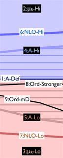
By default, VINCIA also adds a pane below the main plot showing the relative
decomposition of the total variation into its components.
A legend for this pane is given in the illustration here to the right, with names corresponding to VINCIA's automatic uncertainties and numbers indicating the vector index. As an aid to visualizing the many possible contributions, blue colours are used for even vector indices (generally corresponding to "High" variations in VINCIA) and red ones for odd indices (generally corresponding to "Low" variations in VINCIA),
with the exception of index numbers 1, 8, and 9 which are drawn as black lines.
The y axis of the relative-uncertainty pane goes from -1 to 1.
Above (below) zero, each variation
greater than (smaller than) the central one is shown expressed as a fraction of
the largest (smallest) variation. Thus, this pane illustrates, bin by bin,
which source of uncertainty generates the largest contribution to the total.
Due to unitarity, one generally sees a cross-over between reds and blues at the intersection
between Sudakov- and hard-radiaton-dominated regions.
mode LiveDisplays:optStat
(default = 0)
Option to include the ROOT optStat information on plots.
flag LiveDisplays:verbose
(default = off)
Option to enable verbose (e.g., debug) output from LiveDisplays.
Example Programs
The following example programs are included with the VINCIA
distribution and illustrate how to use the ROOT
interface:
vincia03-root.cc : create and save
runtime displays, including comparisons to files containing
experimental data points in a variety of formats. vincia04-root.cc : save ROOT
histograms to a ROOT file, eg for later manipulation and/or custom plotting.vincia05-root.cc : save the output of a previous run
to a histogram file and overplot it on the current one.vincia07-root.cc : using the runtime displays to plot ratios of
VINCIA radiation functions to MADGRAPH matrix
elements. vincia08-root.cc : run
several PYTHIA and VINCIA instances concurrently, plotting the
results of all them simultaneously.vincia10-root.cc : run
several centre-of-mass energies,
plotting how various quantities scale with energy.